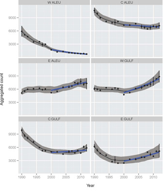
Figure 1. Estimated regional trends of Steller sea lion aerial survey counts in the wDPS. The blue line represents the fitted trend for each region from 2000 to 2012 and the gray envelope represents the total augmented counts over each site within the separate regions. The points are the regional total of each count plus the augmented data. The error bars represent the variation in the observed counts plus the augmented data. Plot titles correspond to regions of the Aleutian Islands and Gulf of Alaska, e.g., W ALEU=Western Aleutian Islands, C ALEU=Central Aleutian Islands, and E GULF=Eastern Gulf of Alaska.
Part of the NMFS' mission is to monitor populations of Steller sea lions (Eumetopias jubatus). Estimating trends in growth is a central tenet in managing ecological populations and there are many methods for estimating general population trends. The most common include simple linear regression of log-abundance, state-space modeling, and Bayesian hierarchical modeling.
While all of these methods have benefits, they have one downfall that is a major stumbling block for Steller sea lion monitoring: trend is estimated from a single parameter in the model. Thus, estimating regional trends in sea lion abundance can prove difficult if the many survey sites are not surveyed in a single year.
The National Marine Mammal Laboratory's Alaska Ecosystems Program (AEP) proposed a methodology and software to overcome this problem by treating a trend as a summary of abundance, rather than a model parameter. To make this method widely available for future sea lion monitoring, as well as to other ecologists in general, we created the add-on package agTrend for the R statistical environment (R Development Core Team 2013).
The package is freely available from the project website http://nmml.github.io/agTrend. Users can find links and directions for installation.
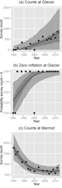
Figure 2. Predicted survey counts at the Glacier haul out and Marmot rookery. The dark and light grey envelopes are the 50th and 90th percentiles for the simulation distribution, respectively. For plots (a) and (c), the points are the observed counts; while for plot (b), the points are indicators of positive counts. The black line is the median augmented counts for (a) and (c); while in (b), it is the median probability of a positive count.
In the AEP's Steller sea lion monitoring studies, aggregating site-level abundance into regional abundance is problematic because sites may not be surveyed in the same years. So, site-level abundance cannot simply be "summed up" to form regional abundance observations. Moreoverbecause sea lion monitoring has been going on for more than 20 yearssurvey methods have changed, prohibiting direct comparison of abundance across years. For example, in the 1990s and early 2000s photographs of sea lion sites were taken with handheld cameras during aerial surveys. Beginning in 2004, photographs were taken with high-resolution, belly-mounted cameras on the survey plane.
Hierarchical models can be used to estimate regional-level trends and correct for changing methodology; however, the resulting inference is interpreted as the average trend, which is not the same as the trend of the regional total abundance.
To circumvent this problem, we took an approach using Bayesian Markov Chain Monte Carlo (MCMC) methods and a hierarchical model to augment missing site data.
After the missing data is simulated, forming regional sums of abundance over many sites is straightforward. The augmentation procedure used by agTrend is based on two hierarchical processes, the observation process and the abundance process. The observation model accounts for changes in survey methodology or environmental conditions over the course of the monitoring program that affect the observed sea lion aerial survey observations. The abundance process models the normalized sea lion counts.
The normalized abundance refers to the count that would be observed had the surveys been conducted under what could be termed "ideal" conditions. The normalization allows for proper comparisons of sea lion counts across years. The basic procedure is to simulate realizations of the normalized sea lion counts at every site, then sum the values over regions of interest, and finally, the trend in abundance is calculated for each simulation. We then summarize the distribution of simulated trends to form estimates of regional Steller sea lion trends.
The agTrend package includes several demonstration scripts for analyzing Steller sea lion aerial survey data. Figure 1 illustrates estimated trend lines (2000-12) and augmented data for a regional aggregation of Steller sea lion aerial survey counts in the western Distinct Population Segment (wDPS; sites west of 144°W longitude). The estimates of trend in aerial survey counts from this analysis are provided in Table 1.
Data augmentation for individual sites is illustrated in Figure 2. Figure 2 also illustrates another technical challenge of trend estimation for Steller sea lions, observed counts of zero at some sites in some years. To model this phenomenon, a zero-inflated abundance model can be used for some sites. In Figure 2, (a) shows the augmented aerial counts for the Glacier Island haul-out site, (b) shows the estimated probability of observing zero animals in any given survey year, and (c) illustrates the data augmentation for the Marmot Island rookery, a large site with essentially zero probability of observing an empty beach.
Table 1. Regional trend estimates for 2000-12. The trend estimates are given in percent growth form. The columns are the simulated median and the lower and upper 95th percentiles.