Ecosystem IndicatorsNoteworthy Topics (pdf)Quantifying Linkages Among Report Card IndicatorsEcosystem Status Reports (ESRs) compile a wide range of ecosystem indicators and also include qual- itative assessments based on current-year indicators that reflect the status and trends of ecosystem components, from physical oceanography to fishes and seabirds. Each ESR also includes a Report Card (see Figure 2 which is a subset of indicators intended to capture main components of the ecosystem. For each Report Card indicator, the mean and trend over the most recent five years are displayed. For more information on the methods for plotting the Report Card indicators, please see ‘Methods Description for the Report Card Indicators’ (p. 241). Exploring quantitative linkages among Report Card indicators illustrates how changes in one variable might affect another (i.e., which indicators are stronger/weaker determinants of trends in other ecosys- tem components). The method proposed here, dynamic structural equation modeling, can also project next year values and can therefore be used as a tool alongside the Spring PEEC (Preview of Ecosystem and Economic Conditions) meeting to identify emergent trends and potential noteworthy topics to track through summer surveys and research efforts. Understanding ecosystem structure and function usually begins by organizing indicators within a simpli- fied conceptual model, such that ecological relationships among indicators can be expressed, visualized, and discussed. One simplified approach to visualize relationships among variables is a qualitative network model (QNM) (Levins, 1974). QNMs summarize the relationship among multiple variables (represented as boxes) that are linked by hypothesized mechanisms (represented as arrows), where mechanisms are specified as a positive or negative impact of one variable on another. QNMs have been successfully used at the Alaska Fisheries Science Center to identify likely consequences of hypothetical ecosystem changes (Reum et al., 2015, 2021), and can incorporate stakeholder input regarding relevant variables (boxes) and mechanisms (arrows). Extending QNMs, we develop a time-series model that includes ecosystem indicators (boxes) and hy- pothesized linkages (arrows), where the strength of linkage can either be specified a priori (i.e., specifying that a 10% increase in a predator drives a 10% decrease in per-capita production for a prey species) or estimated from available time-series data. This approach - dynamic structural equation modeling (DSEM) - has been demonstrated via application to recruitment modeling for walleye pollock (among other uses) (Thorson et al., in review). DSEM can accommodate a combination of lagged and simul- taneous impacts of any variable on any other variable and jointly estimates the strength of impacts (termed “path coefficients”). Additionally, DSEM can estimate missing values within indicator time series, thereby accommodating biennial survey structures, for example. DSEM also addresses potential correlations and complementarity (i.e., trade-offs) among indicators. We specifically propose a DSEM linking Report Card indicators included in this eastern Bering Sea Ecosystem Status Report. The specified structure for this DSEM is based upon the following design choices:
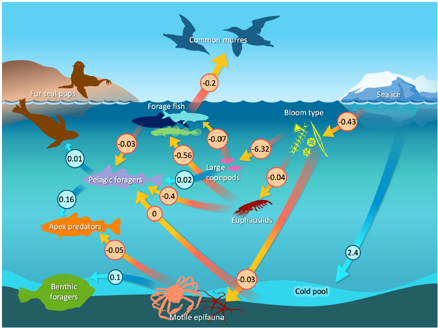
Fitting this conceptual model to time-series data (Figure 3) results in some linkages that are in-line with prior expectations. For example, increased sea ice drives an increase in cold pool extent and a decrease in the proportion of open water blooms. Open-water blooms in turn cause a decrease in motile epifauna and benthic foragers. Periods with more open water blooms are also estimated to cause a decrease in large copepods (because the Report Card time-series show a negative correlation between “Bloom.Type” and “Large.Copepod” indicators). On the other hand, model results also show some linkages that are not consistent with prior expectations. For example, increased euphausiid abundance is estimated to decrease both forage fish and pelagic forager abundance. Similarly, increased forage fish is estimated to decrease the reproductive success of fish-eating seabirds. Finally, we note that DSEM provides interpolated estimates of Report Card indicators in years that are otherwise missing direct measurements (Figure 4). These interpolated estimates seem reasonable in many cases. For example, euphausiid measurements are high in the mid-2000s and low by the mid-2010s, and show relatively little variation around this dominant trend. The model then estimates a high auto-correlation, and interpolates values (and associated uncertainty) that are consistent with this dominant pattern. By contrast, forage fishes show larger interannual variation, so interpolated values are then estimated with greater uncertainty. DSEM also provides ‘historical projections’ of Report Card indicators earlier than their first observation. These hindcasts assume that ecosystem dynamics are stationary, analogous to how climate projections are constructed for future decades. However, we do not show these historical projections prior to 1982 for variables without a direct measurement. We conclude that DSEM provides an avenue to combine a conceptual model for ecosystem function with time-series indicators that are compiled in the ESRs, while compensating for (and interpolating) missing data. We foresee that future research during 2024 could address some estimated linkages that are currently inconsistent with widely understood relationships. For example, we could separate forage fish into taxa with better understood linkages with other variables (e.g., separating cold-associated capelin from warm-associated herring). We also note that estimated linkages involving euphausiids are surprising and generally conflict with assumed dynamics. This suggests that more empirical research is needed to measure euphausiid abundance and consumption to link changes in these variables to both oceanography as well as changes in predator abundance. Contributed by James Thorson1 and Elizabeth Siddon2 Indicators provided by Lewis A.K. Barnett1, David Kimmel1, Jens M. Nielsen1,3, Patrick H. Ressler1, Sean Rohan1, Matthew Rustand4, Rick Thoman5, Rodney Towell1, George A. Whitehouse1,3, and Ellen M. Yasumiishi2 Methods development 1NOAA Fisheries, Alaska Fisheries Science Center, Seattle, WA
Figure 3: A path diagram showing estimated quantitative linkages among ecosystem variables. Arrows correspond to hypothesized relationships, where an arrow pointing from X to Y indicates that a change in X is estimated to cause a change in Y and the number next to each arrow shows the estimated magnitude (using red arrows to indicate negative and blue arrows to indicate positive effects). Each path coefficient also estimates the statistical significance of that hypothesized mechanism (values not shown here to avoid clutter) and future research could conduct model-selection to eliminate non-significant linkages. 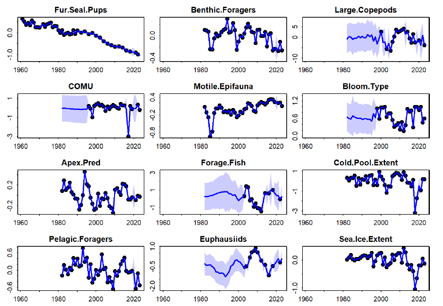 Figure 4: Observed (black dot) and estimated (blue line with 95% confidence interval as shaded area) value for each ecosystem variable included in the Dynamic Structural Equation Model. |

EBS Noteworthy 2023