|
Research on Incorporating Environmental Data Within Stock
Assessments:
Bering Sea Pollock
by Jim Ianelli
A large body of research on
changes in the physical environment of the North
Pacific Ocean is ongoing at the AFSC in
collaboration with oceanographers at several
institutions. Within the Center, scientists
have pursued application of the Ocean Surface
Current Simulations (OSCURS) model to describe
changes in the Bering Sea that may have affected
early-life conditions of walleye pollock. The
OSCURS model represents a drift-simulator that uses
sea-level pressure data to predict surface current
movements. The observed pressure data are used
to derive wind characteristics and obtain measures
of drift from arbitrary locations in the ocean.
Arsenev (1967) presented drift patterns for
the Bering Sea based on limited drift observations
from Soviet research vessels during the 1960s.
Direct observation of drift has been shown to
be consistent with the magnitude and type of pattern
expected based on simulations from the OSCURS model.
To enhance the description of Arsenev, we conducted
OSCURS model runs from each month over a grid of
points throughout the eastern Bering Sea from 1960
to 2000. Computing the monthly average over
these years, a “climatology” of surface currents
indicates strong seasonal shifts (see
Figure 1). The degree to which these
seasonal patterns affect pollock abundance
distribution and survival is an ongoing research
project at the AFSC in collaboration with other
climate and oceanographic research groups.
In addition to describing the general
patterns of surface currents within the Bering Sea,
these analyses provide the ability to scrutinize the
degree of interannual variability in surface
advection patterns that may affect larval-adult
separation and cannibalism. For example,
examining the current patterns for April in
different years gives some indication of the kind of
interannual variability in current patterns (see
Figure 2). Given alternative
hypotheses on the importance of different spawning
distributions, these patterns provide insight into
factors that may lead to high survival levels for
eggs and larvae. Advection in the months
subsequent to peak spawning (e.g., April) may also
provide a good indication of movement of eggs and
larvae into prime nursery areas. To date,
implementation of an advection model within the
stock assessment model has had relatively little
impact on values critical for harvest management
regulations but has explained a large part of the
interannual variability in pollock recruitment.
| |
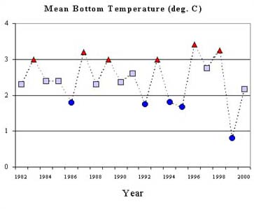
 Figure 3. Mean summer bottom temperatures used
to model bottom trawl survey pollock catchability,
1982-2000. Triangles represent years
classified as "warm", squares as
"intermediate", and circles as
"cold" temperature years. (Note:
these were normalized to have mean zero for use in
the model).
|
In addition to evaluating the overall geographic
concentrations of pollock over time, these data were
further broken down by length and age. In
general, smaller fish are more common in the
northern areas of the eastern Bering Sea with
apparent movement towards the south and east as the
pollock become larger. These patterns are also
revealed when one computes the centers of abundance
based on age-specific CPUE (catch-per-unit-effort)
data. This is done by simply computing the CPUE-weighted average location for specific ages.
Because bottom temperature has long been
considered important in the distribution of pollock
on the shelf (e.g., the Southeast Bering Sea
Carrying Capacity), we pooled over years into
three categories: cold (< 2°C ), intermediate
(2° - 3°C ), and warm ( >= 3°C) based on the
mean bottom temperature (Figure 3). (See
related report “Spatial
Distribution and Ontogenetic Movement of Walleye
Pollock in the Eastern Bering Sea” in this
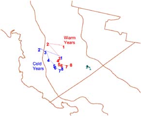
section.) The average locations for warm years are
farther on-shelf than for cold years indicating a
broader dispersal onto the shelf in warmer years.
The average locations for intermediate years
were not depicted here, but were most similar to the
cold years. The mean centers of distribution
in both warm and cold years have very similar
patterns with age. Younger fish are found to
the north and northwestern regions and as they age,
the centers of distribution move south and
southeasterly.
| |

Figure 4. EBS pollock weighted (by number)
average location by ages 1-8, 1982-2000. Lower
left line represents the average from
"cold" years while the upper right line
represents average location during "warm"
years. Triangles represent the centers of
survey operations in each year.
|
Bottom temperature data collected during NMFS summer
bottom-trawl surveys were used within the stock
assessment model. Based on age-specific
estimates of centers-of-distribution, it appears
that temperature affects the distribution of pollock
on the shelf (Figure 4). It therefore
seems likely that temperature may affect the
availability of the stock to the survey. That
is, temperature may affect the proportion of the
stock that is within or outside of the standard
survey area. We therefore evaluate this
potential as an effect on the survey catchability in
year t base on temperature Tt
as:
qt
= μq + βqTt
Where μq is the
mean catchability and βq
represents the slope parameter. The time
series of temperature (Figure 3 above) is used in a
model alternate for this year's assessment.
| |

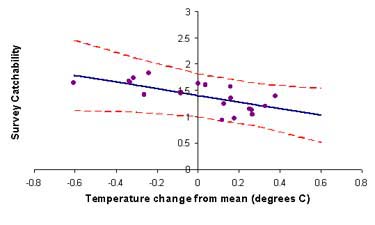
Figure 5. Estimated relationship between
pollock bottom-trawl
survey catchability and bottom temperature
|
Results suggest that there is a slight negative
relationship between bottom temperatures and survey
catchability (slope -0.631, with standard error
0.363). Based on this relationship, survey
catchability tends to be lower at warmer
temperatures and slightly higher at colder
temperatures (Figure 5 below). In other words,
in cold years pollock appear to be more available to
the survey gear than in warm years.
Additional research investigating the mechanism for
the apparent effect of bottom temperature on survey
catchability/availability is ongoing. One
hypothesis is that during colder years, pollock are
more prevalent on the bottom than in warm
years. Alternatively, their overall
distribution may be different (i.e., fall further
outside of the standard survey area during warmer
years).
Next >>>

|

|
quarterly Oct-Dec 2001 sidebar
AFSC Quarterly
Research Reports
Oct-Dec 2001
Contents
Feature
Auke Bay Lab
National Marine
Mammal Lab
RACE Division
REFM Division
Items
Quarterly Index
Quarterly Home
|

